Aug 18, 2014

Microsoft Excel comes with a whole heap of different chart types and it is amazing to see that Waterfall chart is not one of them. A Waterfall chart is a column chart that only shows the growth in each row of data. Therefore, we should make one manually if need be. To do this, we need to create a new table out of the original that shows the growth for each row, and then simply chart this new table. Let’s say that we need to create a Waterfall chart for a table that holds student scores. Here are the steps you’d take to create this chart. Step 1: Copy the table to a separate sheet.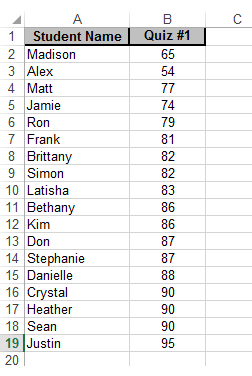 Step 2: In the new table delete column B and in cell B2, type ‘0’ (zero). 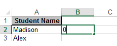Step 3: In cell B3, type the formula =Data!B2, where ‘Data’ is the name of the sheet containing the original table and ‘B2’ is the cell reference which is one above the reference of the current cell. So for Alex, we put Madison’s score. 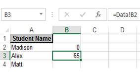Step 4: Autofill the formula in cell B3 down so it’s copied all the way to the end of the table. 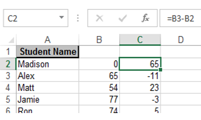Step 5: In cell C2 type, =B3-B2 and autofill down. This generates the growth value for each row. Step 6: In cell D2 type, =B2. Then in cell, D3 type =IF(C3<0, B3+C3,B3) and again, autofill downwards. 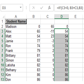Step 7: In cell E2 type, =ABS(C2) and autofill downwards. The ABS() function returns the Absolute Value of a number. Also, label column E as “Growth,” or something similar. 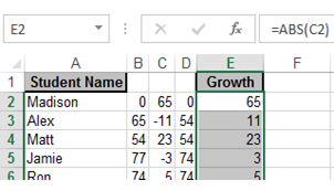Step 8: You are now ready to chart the table. Since you don’t need to use columns B and C, you can hide them if you want but don’t delete them as they are being used in the formulas. Step 9: Select the whole table and from your Ribbon, click on the ‘Insert,’ select the ‘Chart’ group, and under the ‘Column’ option, select ‘Stacked Column.’ 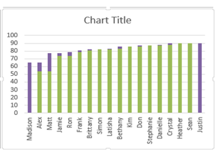Step 10: Click on one of the columns located in the lower part of the stack (shown green in the picture) to select the data series. 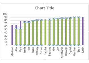Step 11: We now need to hide this data series by choosing a colour that is the same as the background colour. In our case, the colour is white. So from the Ribbon, select ‘Chart Tools,’ click on ‘Format’ and under ‘Shape Fill,’ choose the white colour and click away somewhere to de-select the series. 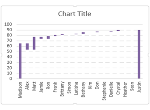Now you can see that the data now flows like a waterfall. We can now add a ‘Chart Title’ or ‘Legend’ to our chart to finish the chart off.