May 18, 2015

You may remember a previous blog post of mine about advanced filters previously. I recently had a student in one of our Excel Courses who was interested in filtering and she wasn't aware of advanced filters. After showing her how to do advanced filters, she asked me if there was a way to speed up finding out how many products came from the list and what the total amount of the specific products sold. I showed her database functions and she was really happy with the result.

What are database functions? 

They are a version of the standard aggregating functions (like SUM, AVERAGE, COUNT, and so on).

So if you like those functions, but you want a ‘more specific’ SUM or you use SUMIF and SUMIFS a lot but find them a little limiting, you’ll love DSUM. There is also DAVERAGE, and DCOUNT of course, if you prefer those.

So, how does it work? Basically, a database function performs an advanced filter (without actually hiding the rows) and then sums (or averages or counts) the result of the advanced filter.

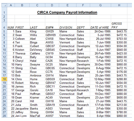
So a quick reminder of advanced filters. An advanced filter needs a criteria area that has the same column headings as the list’s column headings. Here’s the list:

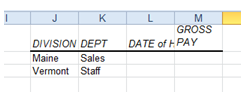
And here is the criteria area (which are the same as in my previous blog post):

When I perform the filter, I get this result:

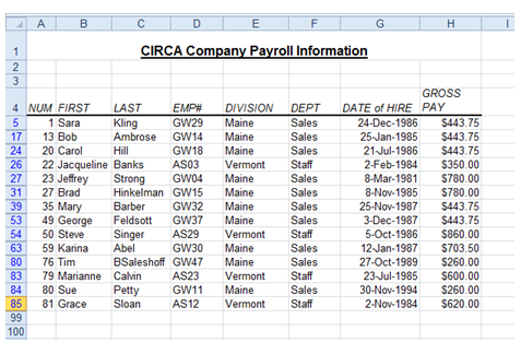
Note, that there are 14 rows and that the total of the gross pays is $7432.25.

I’m going to remove the filter so that all the rows are visible. You don't have to do this, the DSUM will work regardless. Now, I'll click in a blank cell and type in this formula: =DSUM(

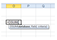
A DSUM has three parts:

1. The database – This is just the list, so for me this is A4 to H98. This includes the heading row, just like you would for an advanced filter.
2. The field – The name of the column in the list that I want to sum up. Here, I'm inputting “GROSS PAY,” which has to be exactly the same word as the heading in the list. (Note: It actually doesn't have be exactly the same case, so I could have put “gross pay” but I like my formulas to not only work, but to also look ‘right’).
3. The criteria – You can probably guess that the criteria area would normally be used in an advanced filter. In my case, this is J1 to M3.

Note: If you have previously performed an advanced filter on the list, the reference for the criteria (J1:M3) may get replaced with the word criteria. This is Excel automatically setting up a range name for us. We can leave it, or type and change it back to the cell reference, the formula will work either way.

So my formula looks like this: =DSUM(A4:H98,”GROSS PAY”,J1:M3)

When I press Enter, we get an answer of $7,432,25. Sound familiar? It’s the same as what the advanced filter gave us.

The really cool advantage of a database function over the advanced filter is that if I change the criteria in the criteria area then the formula automatically updates itself. I don’t have to turn the filter off and then turn it on again!

Hope that helps you with doing your calculations in Excel.